hypothesis vs anova

An open portfolio of interoperable, industry leading products

The Dotmatics digital science platform provides the first true end-to-end solution for scientific R&D, combining an enterprise data platform with the most widely used applications for data analysis, biologics, flow cytometry, chemicals innovation, and more.

Statistical analysis and graphing software for scientists

Bioinformatics, cloning, and antibody discovery software

Plan, visualize, & document core molecular biology procedures

Electronic Lab Notebook to organize, search and share data

Proteomics software for analysis of mass spec data

Modern cytometry analysis platform

Analysis, statistics, graphing and reporting of flow cytometry data

Software to optimize designs of clinical trials

POPULAR USE CASES

The Ultimate Guide to ANOVA

Get all of your ANOVA questions answered here

ANOVA is the go-to analysis tool for classical experimental design, which forms the backbone of scientific research.

In this article, we’ll guide you through what ANOVA is, how to determine which version to use to evaluate your particular experiment, and provide detailed examples for the most common forms of ANOVA.

This includes a (brief) discussion of crossed, nested, fixed and random factors, and covers the majority of ANOVA models that a scientist would encounter before requiring the assistance of a statistician or modeling expert.

What is ANOVA used for?

ANOVA, or (Fisher’s) analysis of variance, is a critical analytical technique for evaluating differences between three or more sample means from an experiment. As the name implies, it partitions out the variance in the response variable based on one or more explanatory factors.

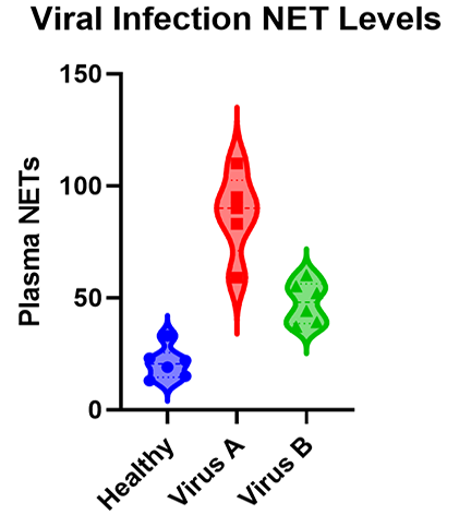
As you will see there are many types of ANOVA such as one-, two-, and three-way ANOVA as well as nested and repeated measures ANOVA. The graphic below shows a simple example of an experiment that requires ANOVA in which researchers measured the levels of neutrophil extracellular traps (NETs) in plasma across patients with different viral respiratory infections.

Many researchers may not realize that, for the majority of experiments, the characteristics of the experiment that you run dictate the ANOVA that you need to use to test the results. While it’s a massive topic (with professional training needed for some of the advanced techniques), this is a practical guide covering what most researchers need to know about ANOVA.

When should I use ANOVA?

If your response variable is numeric, and you’re looking for how that number differs across several categorical groups, then ANOVA is an ideal place to start. After running an experiment, ANOVA is used to analyze whether there are differences between the mean response of one or more of these grouping factors.

ANOVA can handle a large variety of experimental factors such as repeated measures on the same experimental unit (e.g., before/during/after).

If instead of evaluating treatment differences, you want to develop a model using a set of numeric variables to predict that numeric response variable, see linear regression and t tests .

What is the difference between one-way, two-way and three-way ANOVA?

The number of “ways” in ANOVA (e.g., one-way, two-way, …) is simply the number of factors in your experiment.

Although the difference in names sounds trivial, the complexity of ANOVA increases greatly with each added factor. To use an example from agriculture, let’s say we have designed an experiment to research how different factors influence the yield of a crop.

An experiment with a single factor

In the most basic version, we want to evaluate three different fertilizers. Because we have more than two groups, we have to use ANOVA. Since there is only one factor (fertilizer), this is a one-way ANOVA. One-way ANOVA is the easiest to analyze and understand, but probably not that useful in practice, because having only one factor is a pretty simplistic experiment.

What happens when you add a second factor? 

If we have two different fields, we might want to add a second factor to see if the field itself influences growth. Within each field, we apply all three fertilizers (which is still the main interest). This is called a crossed design. In this case we have two factors, field and fertilizer, and would need a two-way ANOVA.

As you might imagine, this makes interpretation more complicated (although still very manageable) simply because more factors are involved. There is now a fertilizer effect, as well as a field effect, and there could be an interaction effect, where the fertilizer behaves differently on each field.

How about adding a third factor?

Finally, it is possible to have more than two factors in an ANOVA. In our example, perhaps you also wanted to test out different irrigation systems. You could have a three-way ANOVA due to the presence of fertilizer, field, and irrigation factors. This greatly increases the complication.

Now in addition to the three main effects (fertilizer, field and irrigation), there are three two-way interaction effects (fertilizer by field, fertilizer by irrigation, and field by irrigation), and one three-way interaction effect.

If any of the interaction effects are statistically significant, then presenting the results gets quite complicated. “Fertilizer A works better on Field B with Irrigation Method C ….”

In practice, two-way ANOVA is often as complex as many researchers want to get before consulting with a statistician. That being said, three-way ANOVAs are cumbersome, but manageable when each factor only has two levels.

What are crossed and nested factors?

In addition to increasing the difficulty with interpretation, experiments (or the resulting ANOVA) with more than one factor add another level of complexity, which is determining whether the factors are crossed or nested.

With crossed factors, every combination of levels among each factor is observed. For example, each fertilizer is applied to each field (so the fields are subdivided into three sections in this case).

With nested factors, different levels of a factor appear within another factor. An example is applying different fertilizers to each field, such as fertilizers A and B to field 1 and fertilizers C and D to field 2. See more about nested ANOVA here .

What are fixed and random factors?

Another challenging concept with two or more factors is determining whether to treat the factors as fixed or random. 

Fixed factors are used when all levels of a factor (e.g., Fertilizer A, Fertilizer B, Fertilizer C) are specified and you want to determine the effect that factor has on the mean response. 

Random factors are used when only some levels of a factor are observed (e.g., Field 1, Field 2, Field 3) out of a large or infinite possible number (e.g., all fields), but rather than specify the effect of the factor, which you can’t do because you didn’t observe all possible levels, you want to quantify the variability that’s within that factor (variability added within each field).

Many introductory courses on ANOVA only discuss fixed factors, and we will largely follow suit other than with two specific scenarios (nested factors and repeated measures). 

What are the (practical) assumptions of ANOVA?

These are one-way ANOVA assumptions, but also carryover for more complicated two-way or repeated measures ANOVA.

• Categorical treatment or factor variables - ANOVA evaluates mean differences between one or more categorical variables (such as treatment groups), which are referred to as factors or “ways.”
• Three or more groups - There must be at least three distinct groups (or levels of a categorical variable) across all factors in an ANOVA. The possibilities are endless: one factor of three different groups, two factors of two groups each (2x2), and so on. If you have fewer than three groups, you can probably get away with a simple t-test.
• Numeric Response - While the groups are categorical, the data measured in each group (i.e., the response variable) still needs to be numeric. ANOVA is fundamentally a quantitative method for measuring the differences in a numeric response between groups. If your response variable isn’t continuous, then you need a more specialized modelling framework such as logistic regression or chi-square contingency table analysis to name a few.
• Random assignment - The makeup of each experimental group should be determined by random selection.
• Normality - The distribution within each factor combination should be approximately normal, although ANOVA is fairly robust to this assumption as the sample size increases due to the central limit theorem.

What is the formula for ANOVA?

The formula to calculate ANOVA varies depending on the number of factors, assumptions about how the factors influence the model (blocking variables, fixed or random effects, nested factors, etc.), and any potential overlap or correlation between observed values (e.g., subsampling, repeated measures). 

The good news about running ANOVA in the 21st century is that statistical software handles the majority of the tedious calculations. The main thing that a researcher needs to do is select the appropriate ANOVA.

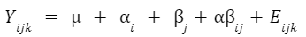
An example formula for a two-factor crossed ANOVA is:

How do I know which ANOVA to use?

As statisticians, we like to imagine that you’re reading this before you’ve run your experiment. You can save a lot of headache by simplifying an experiment into a standard format (when possible) to make the analysis straightforward.

Regardless, we’ll walk you through picking the right ANOVA for your experiment and provide examples for the most popular cases. The first question is:

Do you only have a single factor of interest?

If you have only measured a single factor (e.g., fertilizer A, fertilizer B, .etc.), then use one-way ANOVA . If you have more than one, then you need to consider the following:

Are you measuring the same observational unit (e.g., subject) multiple times?

This is where repeated measures come into play and can be a really confusing question for researchers, but if this sounds like it might describe your experiment, see repeated measures ANOVA . Otherwise:

Are any of the factors nested, where the levels are different depending on the levels of another factor?

In this case, you have a nested ANOVA design. If you don’t have nested factors or repeated measures, then it becomes simple:

Do you have two categorical factors?

Then use two-way ANOVA.

Do you have three categorical factors?

Use three-way ANOVA.

Do you have variables that you recorded that aren’t categorical (such as age, weight, etc.)?

Although these are outside the scope of this guide, if you have a single continuous variable, you might be able to use ANCOVA, which allows for a continuous covariate. With multiple continuous covariates, you probably want to use a mixed model or possibly multiple linear regression.

Prism  does  offer multiple linear regression but assumes that all factors are fixed. A full “mixed model” analysis is not yet available in Prism, but is offered as options within the one- and two-way ANOVA parameters.

How do I perform ANOVA?

Once you’ve determined which ANOVA is appropriate for your experiment, use statistical software to run the calculations. Below, we provide detailed examples of one, two and three-way ANOVA models.

How do I read and interpret an ANOVA table?

Interpreting any kind of ANOVA should start with the ANOVA table in the output. These tables are what give ANOVA its name, since they partition out the variance in the response into the various factors and interaction terms. This is done by calculating the sum of squares (SS) and mean squares (MS), which can be used to determine the variance in the response that is explained by each factor.

If you have predetermined your level of significance, interpretation mostly comes down to the p-values that come from the F-tests. The null hypothesis for each factor is that there is no significant difference between groups of that factor. All of the following factors are statistically significant with a very small p-value.

One-way ANOVA Example

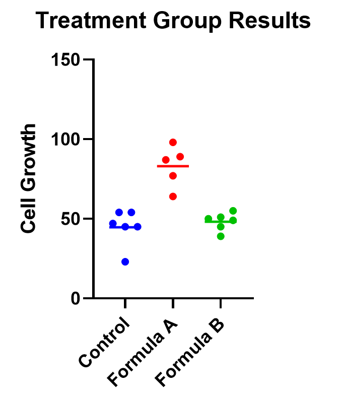
An example of one-way ANOVA is an experiment of cell growth in petri dishes. The response variable is a measure of their growth, and the variable of interest is treatment, which has three levels: formula A, formula B, and a control.

Classic one-way ANOVA assumes equal variances within each sample group. If that isn’t a valid assumption for your data, you have a number of alternatives .

Calculating a one-way ANOVA

Using Prism to do the analysis, we will run a one-way ANOVA and will choose 95% as our significance threshold. Since we are interested in the differences between each of the three groups, we will evaluate each and correct for multiple comparisons (more on this later!). 

For the following, we’ll assume equal variances within the treatment groups. Consider 

The first test to look at is the overall (or omnibus) F-test, with the null hypothesis that there is no significant difference between any of the treatment groups. In this case, there is a significant difference between the three groups (p<0.0001), which tells us that at least one of the groups has a statistically significant difference.

Now we can move to the heart of the issue, which is to determine which group means are statistically different. To learn more, we should graph the data and test the differences (using a multiple comparison correction).

Graphing one-way ANOVA

The easiest way to visualize the results from an ANOVA is to use a simple chart that shows all of the individual points. Rather than a bar chart, it’s best to use a plot that shows all of the data points (and means) for each group such as a scatter or violin plot.

As an example, below you can see a graph of the cell growth levels for each data point in each treatment group, along with a line to represent their mean. This can help give credence to any significant differences found, as well as show how closely groups overlap.

Determining statistical significance between groups

In addition to the graphic, what we really want to know is which treatment means are statistically different from each other. Because we are performing multiple tests, we’ll use a multiple comparison correction . For our example, we’ll use Tukey’s correction (although if we were only interested in the difference between each formula to the control, we could use Dunnett’s correction instead). 

In this case, the mean cell growth for Formula A is significantly  higher  than the control (p<.0001) and Formula B ( p=0.002 ), but there’s no significant difference between Formula B and the control.

Two-way ANOVA example

For two-way ANOVA, there are two factors involved. Our example will focus on a case of cell lines. Suppose we have a 2x2 design (four total groupings). There are two different treatments (serum-starved and normal culture) and two different fields. There are 19 total cell line “experimental units” being evaluated, up to 5 in each group (note that with 4 groups and 19 observational units, this study isn’t balanced). Although there are multiple units in each group, they are all completely different replicates and therefore not repeated measures of the same unit.

As with one-way ANOVA, it’s a good idea to graph the data as well as look at the ANOVA table for results.

Graphing two-way ANOVA

There are many options here. Like our one-way example, we recommend a similar graphing approach that shows all the data points themselves along with the means.

Determining statistical significance between groups in two-way ANOVA

Let’s use a two-way ANOVA with a 95% significance threshold to evaluate both factors’ effects on the response, a measure of growth.

Feel free to use our two-way ANOVA checklist as often as you need for your own analysis.

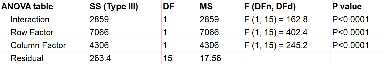
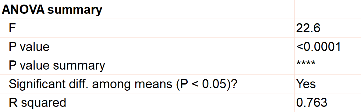
First, notice there are three sources of variation included in the model, which are interaction, treatment, and field. 

The first effect to look at is the interaction term, because if it’s significant, it changes how you interpret the main effects (e.g., treatment and field). The interaction effect calculates if the effect of a factor depends on the other factor. In this case, the significant interaction term (p<.0001) indicates that the treatment effect depends on the field type.

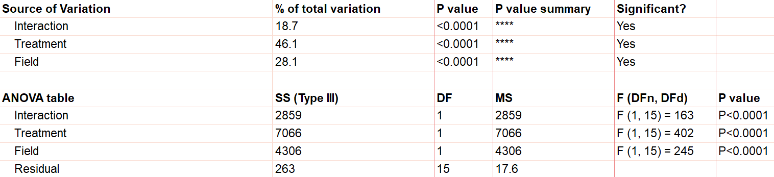
A significant interaction term muddies the interpretation, so that you no longer have the simple conclusion that “Treatment A outperforms Treatment B.” In this case, the graphic is particularly useful. It suggests that while there may be some difference between three of the groups, the precise combination of serum starved in field 2 outperformed the rest.

To confirm whether there is a statistically significant result, we would run pairwise comparisons (comparing each factor level combination with every other one) and account for multiple comparisons.

Do I need to correct for multiple comparisons for two-way ANOVA?

If you’re comparing the means for more than one combination of treatment groups, then absolutely! Here’s more information about multiple comparisons for two-way ANOVA .

Repeated measures ANOVA

So far we have focused almost exclusively on “ordinary” ANOVA and its differences depending on how many factors are involved. In all of these cases, each observation is completely unrelated to the others. Other than the combination of factors that may be the same across replicates, each replicate on its own is independent.

There is a second common branch of ANOVA known as repeated measures . In these cases, the units are related in that they are matched up in some way. Repeated measures are used to model correlation between measurements within an individual or subject. Repeated measures ANOVA is useful (and increases statistical power) when the variability within individuals is large relative to the variability among individuals.

It’s important that all levels of your repeated measures factor (usually time) are consistent. If they aren’t, you’ll need to consider running a mixed model, which is a more advanced statistical technique.

There are two common forms of repeated measures:

• You observe the same individual or subject at different time points. If you’re familiar with paired t-tests, this is an extension to that. (You can also have the same individual receive all of the treatments, which adds another level of repeated measures.)
• You have a randomized block design, where matched elements receive each treatment. For example, you split a large sample of blood taken from one person into 3 (or more) smaller samples, and each of those smaller samples gets exactly one treatment.

Repeated measures ANOVA can have any number of factors. See analysis checklists for one-way repeated measures ANOVA and two-way repeated measures ANOVA .

What does it mean to assume sphericity with repeated measures ANOVA?

Repeated measures are almost always treated as random factors, which means that the correlation structure between levels of the repeated measures needs to be defined. The assumption of sphericity means that you assume that each level of the repeated measures has the same correlation with every other level.

This is almost never the case with repeated measures over time (e.g., baseline, at treatment, 1 hour after treatment), and in those cases, we recommend not assuming sphericity. However, if you used a randomized block design, then sphericity is usually appropriate .

Example two-way ANOVA with repeated measures

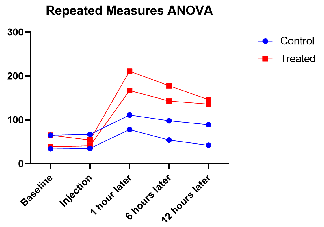
Say we have two treatments (control and treatment) to evaluate using test animals. We’ll apply both treatments to each two animals (replicates) with sufficient time in between the treatments so there isn’t a crossover (or carry-over) effect. Also, we’ll measure five different time points for each treatment (baseline, at time of injection, one hour after, …). This is repeated measures because we will need to measure matching samples from the same animal under each treatment as we track how its stimulation level changes over time.

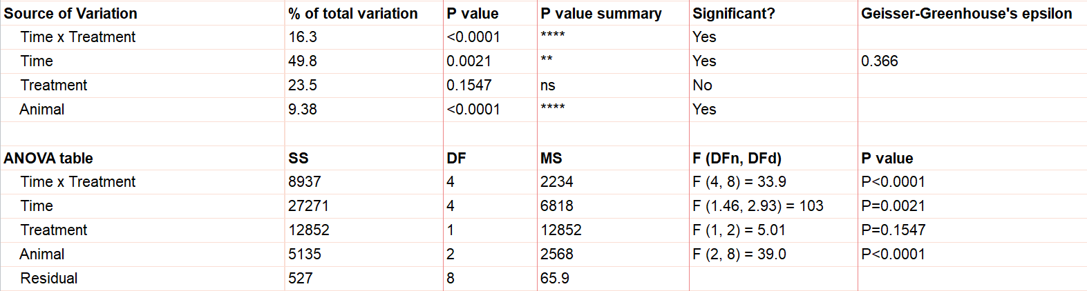
The output shows the test results from the main and interaction effects. Due to the interaction between time and treatment being significant (p<.0001), the fact that the treatment main effect isn’t significant (p=.154) isn’t noteworthy.

Graphing repeated measures ANOVA

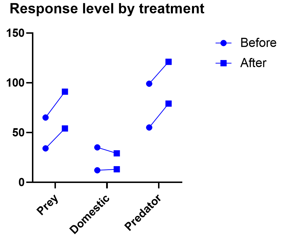
As we’ve been saying, graphing the data is useful, and this is particularly true when the interaction term is significant. Here we get an explanation of why the interaction between treatment and time was significant, but treatment on its own was not. As soon as one hour after injection (and all time points after), treated units show a higher response level than the control even as it decreases over those 12 hours. Thus the effect of time depends on treatment. At the earlier time points, there is no difference between treatment and control.

Graphing repeated measures data is an art, but a good graphic helps you understand and communicate the results. For example, it’s a completely different experiment, but here’s a great plot of another repeated measures experiment with before and after values that are measured on three different animal types.

What if I have three or more factors?

Interpreting three or more factors is very challenging and usually requires advanced training and experience . 

Just as two-way ANOVA is more complex than one-way, three-way ANOVA adds much more potential for confusion. Not only are you dealing with three different factors, you will now be testing seven hypotheses at the same time. Two-way interactions still exist here, and you may even run into a significant three-way interaction term.

It takes careful planning and advanced experimental design to be able to untangle the combinations that will be involved ( see more details here ). 

Non-parametric ANOVA alternatives

As with t-tests (or virtually any statistical method), there are alternatives to ANOVA for testing differences between three groups. ANOVA is means-focused and evaluated in comparison to an F-distribution. 

The two main non-parametric cousins to ANOVA are the Kruskal-Wallis and Friedman’s tests. Just as is true with everything else in ANOVA, it is likely that one of the two options is more appropriate for your experiment.

Kruskal-Wallis tests the difference between medians (rather than means) for 3 or more groups. It is only useful as an “ordinary ANOVA” alternative, without matched subjects like you have in repeated measures. Here are some tips for interpreting Kruskal-Wallis test results. 

Friedman’s Test is the opposite, designed as an alternative to repeated measures ANOVA with matched subjects. Here are some tips for interpreting Friedman's Test . 

What are simple, main, and interaction effects in ANOVA?

Consider the two-way ANOVA model setup that contains two different kinds of effects to evaluate:

The 𝛼 and 𝛽 factors are “main” effects, which are the isolated effect of a given factor. “Main effect” is used interchangeably with “simple effect” in some textbooks.

The interaction term is denoted as “𝛼𝛽”, and it allows for the effect of a factor to depend on the level of another factor. It can only be tested when you have replicates in your study. Otherwise, the error term is assumed to be the interaction term.

What are multiple comparisons?

When you’re doing multiple statistical tests on the same set of data, there’s a greater propensity to discover statistically significant differences that aren’t true differences. Multiple comparison corrections attempt to control for this, and in general control what is called the familywise error rate. There are a number of multiple comparison testing methods , which all have pros and cons depending on your particular experimental design and research questions.

What does the word “way” mean in one-way vs two-way ANOVA?

In statistics overall, it can be hard to keep track of factors, groups, and tails. To the untrained eye “two-way ANOVA” could mean any of these things.

The best way to think about ANOVA is in terms of factors or variables in your experiment. Suppose you have one factor in your analysis (perhaps “treatment”). You will likely see that written as a one-way ANOVA. Even if that factor has several different treatment groups, there is only one factor, and that’s what drives the name. 

Also, “way” has absolutely nothing to do with “tails” like a t-test. ANOVA relies on F tests, which can only test for equal vs unequal because they rely on squared terms. So ANOVA does not have the “one-or-two tails” question .

What is the difference between ANOVA and a t-test?

ANOVA is an extension of the t-test. If you only have two group means to compare, use a t-test. Anything more requires ANOVA.

What is the difference between ANOVA and chi-square?

Chi-square is designed for contingency tables, or counts of items within groups (e.g., type of animal). The goal is to see whether the counts in a particular sample match the counts you would expect by random chance.

ANOVA separates subjects into groups for evaluation, but there is some numeric response variable of interest (e.g., glucose level).

Can ANOVA evaluate effects on multiple response variables at the same time?

Multiple response variables makes things much more complicated than multiple factors. ANOVA (as we’ve discussed it here) can obviously handle multiple factors but it isn’t designed for tracking more than one response at a time. 

Technically, there is an expansion approach designed for this called Multivariate (or Multiple) ANOVA, or more commonly written as MANOVA. Things get complicated quickly, and in general requires advanced training.

Can ANOVA evaluate numeric factors in addition to the usual categorical factors?

It sounds like you are looking for ANCOVA (analysis of covariance). You can treat a continuous (numeric) factor as categorical, in which case you could use ANOVA, but this is a common point of confusion .

What is the definition of ANOVA?

ANOVA stands for analysis of variance, and, true to its name, it is a statistical technique that analyzes how experimental factors influence the variance in the response variable from an experiment.

What is blocking in Anova?

Blocking is an incredibly powerful and useful strategy in experimental design when you have a factor that you think will heavily influence the outcome, so you want to control for it in your experiment. Blocking affects how the randomization is done with the experiment. Usually blocking variables are nuisance variables that are important to control for but are not inherently of interest. 

A simple example is an experiment evaluating the efficacy of a medical drug and blocking by age of the subject. To do blocking, you must first gather the ages of all of the participants in the study, appropriately bin them into groups (e.g., 10-30, 30-50, etc.), and then randomly assign an equal number of treatments to the subjects within each group.

There’s an entire field of study around blocking. Some examples include having multiple blocking variables, incomplete block designs where not all treatments appear in all blocks, and balanced (or unbalanced) blocking designs where equal (or unequal) numbers of replicates appear in each block and treatment combination.

What is ANOVA in statistics?

For a one-way ANOVA test, the overall ANOVA null hypothesis is that the mean responses are equal for all treatments. The ANOVA p-value comes from an F-test.

Can I do ANOVA in R?

While Prism makes ANOVA much more straightforward, you can use open-source coding languages like R as well. Here are some examples of R code for repeated measures ANOVA, both one-way ANOVA in R and two-way ANOVA in R .

Perform your own ANOVA

Are you ready for your own Analysis of variance? Prism makes choosing the correct ANOVA model simple and transparent .

Start your 30 day free trial of Prism   and get access to:

• A step by step guide on how to perform ANOVA
• Sample data to save you time
• More tips on how Prism can help your research

With Prism, in a matter of minutes you learn how to go from entering data to performing statistical analyses and generating high-quality graphs.

Have a language expert improve your writing

Run a free plagiarism check in 10 minutes, generate accurate citations for free.

• Knowledge Base

One-way ANOVA | When and How to Use It (With Examples)

Published on March 6, 2020 by Rebecca Bevans . Revised on May 10, 2024.

ANOVA , which stands for Analysis of Variance, is a statistical test used to analyze the difference between the means of more than two groups.

A one-way ANOVA uses one independent variable , while a two-way ANOVA uses two independent variables.

Table of contents

When to use a one-way anova, how does an anova test work, assumptions of anova, performing a one-way anova, interpreting the results, post-hoc testing, reporting the results of anova, other interesting articles, frequently asked questions about one-way anova.

Use a one-way ANOVA when you have collected data about one categorical independent variable and one quantitative dependent variable . The independent variable should have at least three levels (i.e. at least three different groups or categories).

ANOVA tells you if the dependent variable changes according to the level of the independent variable. For example:

• Your independent variable is social media use , and you assign groups to low , medium , and high levels of social media use to find out if there is a difference in hours of sleep per night .
• Your independent variable is brand of soda , and you collect data on Coke , Pepsi , Sprite , and Fanta to find out if there is a difference in the price per 100ml .
• You independent variable is type of fertilizer , and you treat crop fields with mixtures 1 , 2 and 3 to find out if there is a difference in crop yield .

The null hypothesis ( H 0 ) of ANOVA is that there is no difference among group means. The alternative hypothesis ( H a ) is that at least one group differs significantly from the overall mean of the dependent variable.

If you only want to compare two groups, use a t test instead.

Prevent plagiarism. Run a free check.

ANOVA determines whether the groups created by the levels of the independent variable are statistically different by calculating whether the means of the treatment levels are different from the overall mean of the dependent variable.

If any of the group means is significantly different from the overall mean, then the null hypothesis is rejected.

ANOVA uses the F test for statistical significance . This allows for comparison of multiple means at once, because the error is calculated for the whole set of comparisons rather than for each individual two-way comparison (which would happen with a t test).

The F test compares the variance in each group mean from the overall group variance. If the variance within groups is smaller than the variance between groups , the F test will find a higher F value, and therefore a higher likelihood that the difference observed is real and not due to chance.

The assumptions of the ANOVA test are the same as the general assumptions for any parametric test:

• Independence of observations : the data were collected using statistically valid sampling methods , and there are no hidden relationships among observations. If your data fail to meet this assumption because you have a confounding variable that you need to control for statistically, use an ANOVA with blocking variables.
• Normally-distributed response variable : The values of the dependent variable follow a normal distribution .
• Homogeneity of variance : The variation within each group being compared is similar for every group. If the variances are different among the groups, then ANOVA probably isn’t the right fit for the data.

While you can perform an ANOVA by hand , it is difficult to do so with more than a few observations. We will perform our analysis in the R statistical program because it is free, powerful, and widely available. For a full walkthrough of this ANOVA example, see our guide to performing ANOVA in R .

The sample dataset from our imaginary crop yield experiment contains data about:

• fertilizer type (type 1, 2, or 3)
• planting density (1 = low density, 2 = high density)
• planting location in the field (blocks 1, 2, 3, or 4)
• final crop yield (in bushels per acre).

This gives us enough information to run various different ANOVA tests and see which model is the best fit for the data.

For the one-way ANOVA, we will only analyze the effect of fertilizer type on crop yield.

Sample dataset for ANOVA

After loading the dataset into our R environment, we can use the command aov() to run an ANOVA. In this example we will model the differences in the mean of the response variable , crop yield, as a function of type of fertilizer.

Receive feedback on language, structure, and formatting

Professional editors proofread and edit your paper by focusing on:

• Academic style
• Vague sentences
• Style consistency

See an example

To view the summary of a statistical model in R, use the summary() function.

The summary of an ANOVA test (in R) looks like this:

The ANOVA output provides an estimate of how much variation in the dependent variable that can be explained by the independent variable.

• The first column lists the independent variable along with the model residuals (aka the model error).
• The Df column displays the degrees of freedom for the independent variable (calculated by taking the number of levels within the variable and subtracting 1), and the degrees of freedom for the residuals (calculated by taking the total number of observations minus 1, then subtracting the number of levels in each of the independent variables).
• The Sum Sq column displays the sum of squares (a.k.a. the total variation) between the group means and the overall mean explained by that variable. The sum of squares for the fertilizer variable is 6.07, while the sum of squares of the residuals is 35.89.
• The Mean Sq column is the mean of the sum of squares, which is calculated by dividing the sum of squares by the degrees of freedom.
• The F value column is the test statistic from the F test: the mean square of each independent variable divided by the mean square of the residuals. The larger the F value, the more likely it is that the variation associated with the independent variable is real and not due to chance.
• The Pr(>F) column is the p value of the F statistic. This shows how likely it is that the F value calculated from the test would have occurred if the null hypothesis of no difference among group means were true.

Because the p value of the independent variable, fertilizer, is statistically significant ( p < 0.05), it is likely that fertilizer type does have a significant effect on average crop yield.

ANOVA will tell you if there are differences among the levels of the independent variable, but not which differences are significant. To find how the treatment levels differ from one another, perform a TukeyHSD (Tukey’s Honestly-Significant Difference) post-hoc test.

The Tukey test runs pairwise comparisons among each of the groups, and uses a conservative error estimate to find the groups which are statistically different from one another.

The output of the TukeyHSD looks like this:

First, the table reports the model being tested (‘Fit’). Next it lists the pairwise differences among groups for the independent variable.

Under the ‘$fertilizer’ section, we see the mean difference between each fertilizer treatment (‘diff’), the lower and upper bounds of the 95% confidence interval (‘lwr’ and ‘upr’), and the p value , adjusted for multiple pairwise comparisons.

The pairwise comparisons show that fertilizer type 3 has a significantly higher mean yield than both fertilizer 2 and fertilizer 1, but the difference between the mean yields of fertilizers 2 and 1 is not statistically significant.

When reporting the results of an ANOVA, include a brief description of the variables you tested, the  F value, degrees of freedom, and p values for each independent variable, and explain what the results mean.

If you want to provide more detailed information about the differences found in your test, you can also include a graph of the ANOVA results , with grouping letters above each level of the independent variable to show which groups are statistically different from one another:

If you want to know more about statistics , methodology , or research bias , make sure to check out some of our other articles with explanations and examples.

• Chi square test of independence
• Statistical power
• Descriptive statistics
• Degrees of freedom
• Pearson correlation
• Null hypothesis

Methodology

• Double-blind study
• Case-control study
• Research ethics
• Data collection
• Hypothesis testing
• Structured interviews

Research bias

• Hawthorne effect
• Unconscious bias
• Recall bias
• Halo effect
• Self-serving bias
• Information bias

The only difference between one-way and two-way ANOVA is the number of independent variables . A one-way ANOVA has one independent variable, while a two-way ANOVA has two.

• One-way ANOVA : Testing the relationship between shoe brand (Nike, Adidas, Saucony, Hoka) and race finish times in a marathon.
• Two-way ANOVA : Testing the relationship between shoe brand (Nike, Adidas, Saucony, Hoka), runner age group (junior, senior, master’s), and race finishing times in a marathon.

All ANOVAs are designed to test for differences among three or more groups. If you are only testing for a difference between two groups, use a t-test instead.

A factorial ANOVA is any ANOVA that uses more than one categorical independent variable . A two-way ANOVA is a type of factorial ANOVA.

Some examples of factorial ANOVAs include:

• Testing the combined effects of vaccination (vaccinated or not vaccinated) and health status (healthy or pre-existing condition) on the rate of flu infection in a population.
• Testing the effects of marital status (married, single, divorced, widowed), job status (employed, self-employed, unemployed, retired), and family history (no family history, some family history) on the incidence of depression in a population.
• Testing the effects of feed type (type A, B, or C) and barn crowding (not crowded, somewhat crowded, very crowded) on the final weight of chickens in a commercial farming operation.

In ANOVA, the null hypothesis is that there is no difference among group means. If any group differs significantly from the overall group mean, then the ANOVA will report a statistically significant result.

Significant differences among group means are calculated using the F statistic, which is the ratio of the mean sum of squares (the variance explained by the independent variable) to the mean square error (the variance left over).

If the F statistic is higher than the critical value (the value of F that corresponds with your alpha value, usually 0.05), then the difference among groups is deemed statistically significant.

Quantitative variables are any variables where the data represent amounts (e.g. height, weight, or age).

Categorical variables are any variables where the data represent groups. This includes rankings (e.g. finishing places in a race), classifications (e.g. brands of cereal), and binary outcomes (e.g. coin flips).

You need to know what type of variables you are working with to choose the right statistical test for your data and interpret your results .

Cite this Scribbr article

If you want to cite this source, you can copy and paste the citation or click the “Cite this Scribbr article” button to automatically add the citation to our free Citation Generator.

Bevans, R. (2024, May 09). One-way ANOVA | When and How to Use It (With Examples). Scribbr. Retrieved August 29, 2024, from https://www.scribbr.com/statistics/one-way-anova/

Is this article helpful?

Rebecca Bevans

Other students also liked, two-way anova | examples & when to use it, anova in r | a complete step-by-step guide with examples, guide to experimental design | overview, steps, & examples, what is your plagiarism score.

• Quality Improvement
• Talk To Minitab

Understanding Analysis of Variance (ANOVA) and the F-test

Topics: ANOVA , Hypothesis Testing , Data Analysis

Analysis of variance (ANOVA) can determine whether the means of three or more groups are different. ANOVA uses F-tests to statistically test the equality of means. In this post, I’ll show you how ANOVA and F-tests work using a one-way ANOVA example.

But wait a minute...have you ever stopped to wonder why you’d use an analysis of variance to determine whether means are different? I'll also show how variances provide information about means.

As in my posts about understanding t-tests , I’ll focus on concepts and graphs rather than equations to explain ANOVA F-tests.

What are F-statistics and the F-test?

F-tests are named after its test statistic, F, which was named in honor of Sir Ronald Fisher. The F-statistic is simply a ratio of two variances. Variances are a measure of dispersion, or how far the data are scattered from the mean. Larger values represent greater dispersion.

Variance is the square of the standard deviation. For us humans, standard deviations are easier to understand than variances because they’re in the same units as the data rather than squared units. However, many analyses actually use variances in the calculations.

F-statistics are based on the ratio of mean squares. The term “ mean squares ” may sound confusing but it is simply an estimate of population variance that accounts for the degrees of freedom (DF) used to calculate that estimate.

Despite being a ratio of variances, you can use F-tests in a wide variety of situations. Unsurprisingly, the F-test can assess the equality of variances. However, by changing the variances that are included in the ratio, the F-test becomes a very flexible test. For example, you can use F-statistics and F-tests to test the overall significance for a regression model , to compare the fits of different models, to test specific regression terms, and to test the equality of means.

Using the F-test in One-Way ANOVA

To use the F-test to determine whether group means are equal, it’s just a matter of including the correct variances in the ratio. In one-way ANOVA, the F-statistic is this ratio:

F = variation between sample means / variation within the samples

The best way to understand this ratio is to walk through a one-way ANOVA example.

We’ll analyze four samples of plastic to determine whether they have different mean strengths. (If you don't have Minitab, you can download a free 30-day trial .) I'll refer back to the one-way ANOVA output as I explain the concepts.

In Minitab, choose Stat > ANOVA > One-Way ANOVA...  In the dialog box, choose "Strength" as the response, and "Sample" as the factor. Press OK, and Minitab's Session Window displays the following output: 

Numerator: Variation Between Sample Means

One-way ANOVA has calculated a mean for each of the four samples of plastic. The group means are: 11.203, 8.938, 10.683, and 8.838. These group means are distributed around the overall mean for all 40 observations, which is 9.915. If the group means are clustered close to the overall mean, their variance is low. However, if the group means are spread out further from the overall mean, their variance is higher.

Clearly, if we want to show that the group means are different, it helps if the means are further apart from each other. In other words, we want higher variability among the means.

Imagine that we perform two different one-way ANOVAs where each analysis has four groups. The graph below shows the spread of the means. Each dot represents the mean of an entire group. The further the dots are spread out, the higher the value of the variability in the numerator of the F-statistic.

What value do we use to measure the variance between sample means for the plastic strength example? In the one-way ANOVA output, we’ll use the adjusted mean square (Adj MS) for Factor, which is 14.540. Don’t try to interpret this number because it won’t make sense. It’s the sum of the squared deviations divided by the factor DF. Just keep in mind that the further apart the group means are, the larger this number becomes.

Denominator: Variation Within the Samples

We also need an estimate of the variability within each sample. To calculate this variance, we need to calculate how far each observation is from its group mean for all 40 observations. Technically, it is the sum of the squared deviations of each observation from its group mean divided by the error DF.

If the observations for each group are close to the group mean, the variance within the samples is low. However, if the observations for each group are further from the group mean, the variance within the samples is higher.

In the graph, the panel on the left shows low variation in the samples while the panel on the right shows high variation. The more spread out the observations are from their group mean, the higher the value in the denominator of the F-statistic.

If we’re hoping to show that the means are different, it's good when the within-group variance is low. You can think of the within-group variance as the background noise that can obscure a difference between means.

For this one-way ANOVA example, the value that we’ll use for the variance within samples is the Adj MS for Error, which is 4.402. It is considered “error” because it is the variability that is not explained by the factor.

Ready for a demo of Minitab Statistical Software? Just ask! 

The F-Statistic: Variation Between Sample Means / Variation Within the Samples

The F-statistic is the test statistic for F-tests. In general, an F-statistic is a ratio of two quantities that are expected to be roughly equal under the null hypothesis, which produces an F-statistic of approximately 1.

The F-statistic incorporates both measures of variability discussed above. Let's take a look at how these measures can work together to produce low and high F-values. Look at the graphs below and compare the width of the spread of the group means to the width of the spread within each group.

The low F-value graph shows a case where the group means are close together (low variability) relative to the variability within each group. The high F-value graph shows a case where the variability of group means is large relative to the within group variability. In order to reject the null hypothesis that the group means are equal, we need a high F-value.

For our plastic strength example, we'll use the Factor Adj MS for the numerator (14.540) and the Error Adj MS for the denominator (4.402), which gives us an F-value of 3.30.

Is our F-value high enough? A single F-value is hard to interpret on its own. We need to place our F-value into a larger context before we can interpret it. To do that, we’ll use the F-distribution to calculate probabilities.

F-distributions and Hypothesis Testing

For one-way ANOVA, the ratio of the between-group variability to the within-group variability follows an F-distribution when the null hypothesis is true.

When you perform a one-way ANOVA for a single study, you obtain a single F-value. However, if we drew multiple random samples of the same size from the same population and performed the same one-way ANOVA, we would obtain many F-values and we could plot a distribution of all of them. This type of distribution is known as a sampling distribution .

Because the F-distribution assumes that the null hypothesis is true, we can place the F-value from our study in the F-distribution to determine how consistent our results are with the null hypothesis and to calculate probabilities.

The probability that we want to calculate is the probability of observing an F-statistic that is at least as high as the value that our study obtained. That probability allows us to determine how common or rare our F-value is under the assumption that the null hypothesis is true. If the probability is low enough, we can conclude that our data is inconsistent with the null hypothesis. The evidence in the sample data is strong enough to reject the null hypothesis for the entire population.

This probability that we’re calculating is also known as the p-value!

To plot the F-distribution for our plastic strength example, I’ll use Minitab’s probability distribution plots . In order to graph the F-distribution that is appropriate for our specific design and sample size, we'll need to specify the correct number of DF. Looking at our one-way ANOVA output, we can see that we have 3 DF for the numerator and 36 DF for the denominator.

The graph displays the distribution of F-values that we'd obtain if the null hypothesis is true and we repeat our study many times. The shaded area represents the probability of observing an F-value that is at least as large as the F-value our study obtained. F-values fall within this shaded region about 3.1% of the time when the null hypothesis is true. This probability is low enough to reject the null hypothesis using the common significance level of 0.05. We can conclude that not all the group means are equal.

Learn how to correctly interpret the p-value.

Assessing Means by Analyzing Variation

ANOVA uses the F-test to determine whether the variability between group means is larger than the variability of the observations within the groups. If that ratio is sufficiently large, you can conclude that not all the means are equal.

This brings us back to why we analyze variation to make judgments about means.  Think about the question: "Are the group means different?" You are implicitly asking about the variability of the means. After all, if the group means don't vary, or don't vary by more than random chance allows, then you can't say the means are different. And that's why you use analysis of variance to test the means.

You Might Also Like

• Trust Center

© 2023 Minitab, LLC. All Rights Reserved.

• Terms of Use
• Privacy Policy
• Cookies Settings

What Is An ANOVA Test In Statistics: Analysis Of Variance

Julia Simkus

Editor at Simply Psychology

BA (Hons) Psychology, Princeton University

Julia Simkus is a graduate of Princeton University with a Bachelor of Arts in Psychology. She is currently studying for a Master's Degree in Counseling for Mental Health and Wellness in September 2023. Julia's research has been published in peer reviewed journals.

Learn about our Editorial Process

Saul McLeod, PhD

Editor-in-Chief for Simply Psychology

BSc (Hons) Psychology, MRes, PhD, University of Manchester

Saul McLeod, PhD., is a qualified psychology teacher with over 18 years of experience in further and higher education. He has been published in peer-reviewed journals, including the Journal of Clinical Psychology.

On This Page:

An ANOVA test is a statistical test used to determine if there is a statistically significant difference between two or more categorical groups by testing for differences of means using a variance.

Another key part of ANOVA is that it splits the independent variable into two or more groups.

For example, one or more groups might be expected to influence the dependent variable, while the other group is used as a control group and is not expected to influence the dependent variable.

Assumptions of ANOVA

The assumptions of the ANOVA test are the same as the general assumptions for any parametric test:

• An ANOVA can only be conducted if there is no relationship between the subjects in each sample. This means that subjects in the first group cannot also be in the second group (e.g., independent samples/between groups).
• The different groups/levels must have equal sample sizes .
• An ANOVA can only be conducted if the dependent variable is normally distributed so that the middle scores are the most frequent and the extreme scores are the least frequent.
• Population variances must be equal (i.e., homoscedastic). Homogeneity of variance means that the deviation of scores (measured by the range or standard deviation, for example) is similar between populations.

Types of ANOVA Tests

There are different types of ANOVA tests. The two most common are a “One-Way” and a “Two-Way.”

The difference between these two types depends on the number of independent variables in your test.

One-way ANOVA

A one-way ANOVA (analysis of variance) has one categorical independent variable (also known as a factor) and a normally distributed continuous (i.e., interval or ratio level) dependent variable.

The independent variable divides cases into two or more mutually exclusive levels, categories, or groups.

The one-way ANOVA test for differences in the means of the dependent variable is broken down by the levels of the independent variable.

An example of a one-way ANOVA includes testing a therapeutic intervention (CBT, medication, placebo) on the incidence of depression in a clinical sample.

Note : Both the One-Way ANOVA and the Independent Samples t-Test can compare the means for two groups. However, only the One-Way ANOVA can compare the means across three or more groups.

P Value Calculator From F Ratio (ANOVA)

Two-way (factorial) ANOVA

A two-way ANOVA (analysis of variance) has two or more categorical independent variables (also known as a factor) and a normally distributed continuous (i.e., interval or ratio level) dependent variable.

The independent variables divide cases into two or more mutually exclusive levels, categories, or groups. A two-way ANOVA is also called a factorial ANOVA.

An example of factorial ANOVAs include testing the effects of social contact (high, medium, low), job status (employed, self-employed, unemployed, retired), and family history (no family history, some family history) on the incidence of depression in a population.

What are “Groups” or “Levels”?

In ANOVA, “groups” or “levels” refer to the different categories of the independent variable being compared.

For example, if the independent variable is “eggs,” the levels might be Non-Organic, Organic, and Free Range Organic. The dependent variable could then be the price per dozen eggs.

ANOVA F -value

The test statistic for an ANOVA is denoted as F . The formula for ANOVA is F = variance caused by treatment/variance due to random chance.

The ANOVA F value can tell you if there is a significant difference between the levels of the independent variable, when p < .05. So, a higher F value indicates that the treatment variables are significant.

Note that the ANOVA alone does not tell us specifically which means were different from one another. To determine that, we would need to follow up with multiple comparisons (or post-hoc) tests.

When the initial F test indicates that significant differences exist between group means, post hoc tests are useful for determining which specific means are significantly different when you do not have specific hypotheses that you wish to test.

Post hoc tests compare each pair of means (like t-tests), but unlike t-tests, they correct the significance estimate to account for the multiple comparisons.

What Does “Replication” Mean?

Replication requires a study to be repeated with different subjects and experimenters. This would enable a statistical analyzer to confirm a prior study by testing the same hypothesis with a new sample.

How to run an ANOVA?

For large datasets, it is best to run an ANOVA in statistical software such as R or Stata. Let’s refer to our Egg example above.

Non-Organic, Organic, and Free-Range Organic Eggs would be assigned quantitative values (1,2,3). They would serve as our independent treatment variable, while the price per dozen eggs would serve as the dependent variable. Other erroneous variables may include “Brand Name” or “Laid Egg Date.”

Using data and the aov() command in R, we could then determine the impact Egg Type has on the price per dozen eggs.

ANOVA vs. t-test?

T-tests and ANOVA tests are both statistical techniques used to compare differences in means and spreads of the distributions across populations.

The t-test determines whether two populations are statistically different from each other, whereas ANOVA tests are used when an individual wants to test more than two levels within an independent variable.

Referring back to our egg example, testing Non-Organic vs. Organic would require a t-test while adding in Free Range as a third option demands ANOVA.

Rather than generate a t-statistic, ANOVA results in an f-statistic to determine statistical significance.

What does anova stand for?

ANOVA stands for Analysis of Variance. It’s a statistical method to analyze differences among group means in a sample. ANOVA tests the hypothesis that the means of two or more populations are equal, generalizing the t-test to more than two groups.

It’s commonly used in experiments where various factors’ effects are compared. It can also handle complex experiments with factors that have different numbers of levels.

When to use anova?

ANOVA should be used when one independent variable has three or more levels (categories or groups). It’s designed to compare the means of these multiple groups.

What does an anova test tell you?

An ANOVA test tells you if there are significant differences between the means of three or more groups. If the test result is significant, it suggests that at least one group’s mean differs from the others. It does not, however, specify which groups are different from each other.

Why do you use chi-square instead of ANOVA?

You use the chi-square test instead of ANOVA when dealing with categorical data to test associations or independence between two categorical variables. In contrast, ANOVA is used for continuous data to compare the means of three or more groups.

• Skip to secondary menu
• Skip to main content
• Skip to primary sidebar

Statistics By Jim

Making statistics intuitive

ANOVA Overview

What is anova.

Analysis of variance (ANOVA) assesses the differences between group means. It is a statistical hypothesis test that determines whether the means of at least two populations are different. At a minimum, you need a continuous dependent variable and a categorical independent variable that divides your data into comparison groups to perform ANOVA.

Researchers commonly use ANOVA to analyze designed experiments. In these experiments, researchers use randomization and control the experimental factors in the treatment and control groups. For example, a product manufacturer sets the time and temperature settings in its process and records the product’s strength. ANOVA analyzes the differences in mean outcomes stemming from these experimental settings to estimate their effects and statistical significance. These designed experiments are typically orthogonal, which provides important benefits. Learn more about orthogonality .

Additionally, ANOVA is useful for observational studies . For example, a researcher can observe outcomes for several education methods and use ANOVA to analyze the group differences. However, as with any observational study, you must be careful about the conclusions you draw.

The term "analysis of variance" originates from how the analysis uses variances to determine whether the means are different. ANOVA works by comparing the variance of group means to the variance within groups. This process determines if the groups are part of one larger population or separate populations with different means. Consequently, even though it analyzes variances, it actually tests means! To learn more about this process, read my post, The F-test in ANOVA .

The fundamentals of ANOVA tests are relatively straightforward because it involves comparing means between groups. However, there are an array of elaborations. In this post, I start with the simpler forms and explain the essential jargon. Then I’ll broadly cover the more complex methods.

Simplest Form and Basic Terms of ANOVA Tests

The simplest type of ANOVA test is one-way ANOVA. This method is a generalization of t-tests that can assess the difference between more than two group means.

Statisticians consider ANOVA to be a special case of least squares regression, which is a specialization of the general linear model. All these models minimize the sum of the squared errors.

Related post : The Mean in Statistics

Factors and Factor Levels

To perform the most basic ANOVA, you need a continuous dependent variable and a categorical independent variable. In ANOVA lingo, analysts refer to “categorical independent variables” as factors. The categorical values of a factor are “levels.” These factor levels create the groups in the data. Factor level means are the means of the dependent variable associated with each factor level.

For example, your factor might have the following three levels in an experiment: Control, Treatment 1, and Treatment 2. The ANOVA test will determine whether the mean outcomes for these three conditions (i.e., factor levels) are different.

Related posts : Independent and Dependent Variables and Control Groups in Experiments

Factor Level Combinations

ANOVA allows you to include more than one factor. For example, you might want to determine whether gender and college major correspond to differences in income.

Gender is one factor with two levels: Male and Female. College major is another factor with three levels in our fictional study: Statistics, Psychology, and Political Science.

The combination of these two factors (2 genders X 3 majors) creates the following six groups:

• Male / Statistics
• Female / Statistics
• Male / Psychology
• Female Psychology
• Male / Political Science
• Female / Political Science

These groups are the factor level combinations. ANOVA determines whether the mean incomes for these groups are different.

Factorial ANOVA

ANOVA allows you to assess multiple factors simultaneously. Factorial ANOVA are cases where your data includes observations for all the factor level combinations that your model specifies. For example, using the gender and college major model, you are performing factorial ANOVA if your dataset includes income observations for all six groups.

By assessing multiple factors together, factorial ANOVA allows your model to detect interaction effects. This ability makes multiple factor ANOVA much more efficient. Additionally, evaluating a single factor at a time conceals interaction effects. Single-factor analyses tend to produce inconsistent results when interaction effects exist in an experimental area because they cannot model the interaction effects.

Analysts frequently use factorial ANOVA in experiments because they efficiently test the main and interaction effects for all experimental factors.

Related post : Understanding Interaction Effects

Interpreting the ANOVA Test

ANOVA assesses differences between group means.

Suppose you compare two new teaching methods to the standard practice and want to know if the average test scores for the methods are different. Your factor is Teaching Method, and it contains the following three levels: Standard, Method A, and Method B.

The factor level means are the mean test score associated with each group.

ANOVAs evaluate the differences between the means of the dependent variable for the factor level combinations. The hypotheses for the ANOVA test are the following:

• Null Hypothesis: The group means are all equal.
• Alternative Hypothesis: At least one mean is different.

When the p-value is below your significance level, reject the null hypothesis. Your data favor the position that at least one group mean is different from the others.

While a significant ANOVA result indicates that at least one mean differs, it does not specify which one. To identify which differences between pairs of means are statistically significant, you’ll need to perform a post hoc analysis .

Related post : How to Interpret P Values

General ANOVA Assumptions

ANOVA tests have the same assumptions as other linear models other than requiring a factor. Specifically:

• The dependent variable is continuous.
• You have at least one categorical independent variable (factor).
• The observations are independent.
• The groups should have roughly equal variances (scatter).
• The data in the groups should follow a normal distribution.
• The residuals satisfy the ordinary least squares assumptions .

While ANOVA assumes your data follow the normal distribution, it is robust to violations of this assumption when your groups have at least 15 observations.

ANOVA Designs and Types of Models

The simpler types of ANOVA test are relatively straightforward. However, ANOVA is a flexible analysis, and many elaborations are possible. I’ll start with the simple forms and move to the more complex designs. Click the links to learn more about each type and see examples of them in action!

One-way ANOVA

One-way ANOVA tests one factor that divides the data into at least two independent groups.

Learn about one-way ANOVA and how to perform and interpret an example using Excel.

Two-way ANOVA

Two-way ANOVA tests include two factors that divide the data into at least four factor level combinations. In addition to identifying the factors’ main effects, these models evaluate interaction effects between the factors.

Learn about two-way ANOVA and how to perform and interpret an example using Excel.

Analysis of Covariance (ANCOVA)

ANCOVA models include factors and covariates. Covariates are continuous independent variables that have a relationship with the dependent variable. Typically, covariates are nuisance variables that researchers cannot control during an experiment. Consequently, analysts include covariates in the model to control them statistically.

Learn more about Covariates: Definition and Uses .

Repeated measures ANOVA

Repeated measures designs allow researchers to assess participants multiple times in a study. Frequently, the subjects serve as their own controls and experience several treatment conditions.

Learn about repeated measures ANOVA tests and see an example.

Multivariate analysis of variance (MANOVA)

MANOVA extends the capabilities of ANOVA by assessing multiple dependent variables simultaneously. The factors in MANOVA can influence the relationship between dependent variables instead of influencing a single dependent variable.

There’s even a MANCOVA, which is MANOVA plus ANCOVA! It allows you to include covariates when modeling multiple independent variables.

Learn about MANOVA and see an example.

Crossed and Nested Models

ANOVA can model both crossed and nested factors.

Crossed factors are the more familiar type. Two factors are crossed when each level of a factor occurs with each level of the other factor. The gender and college major factors in the earlier example are crossed because we have all combinations of the factor levels. All levels of gender occur in all majors and vice versa.

A factor is nested in another factor when all its levels occur within only one level of the other factor. Consequently, the data do not contain all possible factor level combinations. For example, suppose you are testing bug spray effectiveness, and your factors are Brand and Product.

In the illustration, Product is nested within Brand because each product occurs within only one level of Brand. There can be no combination that represents Brand 2 and Product A.

The combinations of crossed and nested factors within an ANOVA design can become quite complex!

General Linear Model

The most general form of ANOVA allows you to include all the above and more! In your model, you can have as many factors and covariates as you need, interaction terms, crossed and nested factors, along with specifying fixed, random, or mixed effects, which I describe below.

Types of Effects in ANOVA

Fixed effects.

When a researcher can set the factor levels in an experiment, it is a fixed factor. Correspondingly, the model estimates fixed effects for fixed factors. Fixed effects are probably the type with which you’re most familiar. One-way and two-way ANOVA procedures typically use fixed-effects models. ANOVA models usually assess fixed using ordinary least squares.

For example, in a cake recipe experiment, the researcher sets the three oven temperatures of 350, 400, and 450 degrees for the study. Oven temperature is a fixed factor.

Random effects

When a researcher samples the factor levels from a population rather than setting them, it is a random factor. The model estimates random effects for them. Because random factors sample data from a population, the model must change how it evaluates their effects by calculating variance components .

For example, in studies involving human subjects, Subject is typically a random factor because researchers sample participants from a population.

Mixed effects

Mixed-effects models contain both fixed and random effects. Frequently, mixed-effects models use restricted maximum likelihood (REML) to estimate effects.

For example, a store chain wants to assess sales. The chain chooses five states for its study. State is a fixed factor. Within these states, the chain randomly selects stores. Store is a random factor. It is also nested within the State factor.

Scroll down to find more of my articles about ANOVA!

One Way ANOVA Overview & Example

By Jim Frost Leave a Comment

What is One Way ANOVA?

Use one way ANOVA to compare the means of three or more groups. This analysis is an inferential hypothesis test that uses samples to draw conclusions about populations. Specifically, it tells you whether your sample provides sufficient evidence to conclude that the groups’ population means are different. ANOVA stands for analysis of variance. [Read more…] about One Way ANOVA Overview & Example

ANCOVA: Uses, Assumptions & Example

By Jim Frost 1 Comment

What is ANCOVA?

ANCOVA, or the analysis of covariance, is a powerful statistical method that analyzes the differences between three or more group means while controlling for the effects of at least one continuous covariate. [Read more…] about ANCOVA: Uses, Assumptions & Example

Covariates: Definition & Uses

By Jim Frost 9 Comments

What is a Covariate?

Covariates are continuous independent variables (or predictors) in a regression or ANOVA model. These variables can explain some of the variability in the dependent variable.

That definition of covariates is simple enough. However, the usage of the term has changed over time. Consequently, analysts can have drastically different contexts in mind when discussing covariates. [Read more…] about Covariates: Definition & Uses

How to do Two-Way ANOVA in Excel

By Jim Frost 35 Comments

Use two-way ANOVA to assess differences between the group means that are defined by two categorical factors . In this post, we’ll work through two-way ANOVA using Excel. Even if Excel isn’t your main statistical package, this post is an excellent introduction to two-way ANOVA. Excel refers to this analysis as two factor ANOVA. [Read more…] about How to do Two-Way ANOVA in Excel

How to do One-Way ANOVA in Excel

By Jim Frost 23 Comments

Use one-way ANOVA to test whether the means of at least three groups are different. Excel refers to this test as Single Factor ANOVA. This post is an excellent introduction to performing and interpreting a one-way ANOVA test even if Excel isn’t your primary statistical software package. [Read more…] about How to do One-Way ANOVA in Excel

Using Post Hoc Tests with ANOVA

By Jim Frost 138 Comments

Post hoc tests are an integral part of ANOVA. When you use ANOVA to test the equality of at least three group means, statistically significant results indicate that not all of the group means are equal. However, ANOVA results do not identify which particular differences between pairs of means are significant. Use post hoc tests to explore differences between multiple group means while controlling the experiment-wise error rate.

In this post, I’ll show you what post hoc analyses are, the critical benefits they provide, and help you choose the correct one for your study. Additionally, I’ll show why failure to control the experiment-wise error rate will cause you to have severe doubts about your results. [Read more…] about Using Post Hoc Tests with ANOVA

How F-tests work in Analysis of Variance (ANOVA)

By Jim Frost 51 Comments

Analysis of variance (ANOVA) uses F-tests to statistically assess the equality of means when you have three or more groups. In this post, I’ll answer several common questions about the F-test.

• How do F-tests work?
• Why do we analyze variances to test means ?

I’ll use concepts and graphs to answer these questions about F-tests in the context of a one-way ANOVA example. I’ll use the same approach that I use to explain how t-tests work . If you need a primer on the basics, read my hypothesis testing overview .

To learn more about ANOVA tests, including the more complex forms, read my ANOVA Overview  and One-Way ANOVA Overview and Example .

[Read more…] about How F-tests work in Analysis of Variance (ANOVA)

Benefits of Welch’s ANOVA Compared to the Classic One-Way ANOVA

By Jim Frost 70 Comments

Welch’s ANOVA is an alternative to the traditional analysis of variance (ANOVA) and it offers some serious benefits. One-way analysis of variance determines whether differences between the means of at least three groups are statistically significant. For decades, introductory statistics classes have taught the classic Fishers one-way ANOVA that uses the F-test. It’s a standard statistical analysis, and you might think it’s pretty much set in stone by now. Surprise, there’s a significant change occurring in the world of one-way analysis of variance! [Read more…] about Benefits of Welch’s ANOVA Compared to the Classic One-Way ANOVA

Multivariate ANOVA (MANOVA) Benefits and When to Use It

By Jim Frost 181 Comments

Multivariate ANOVA (MANOVA) extends the capabilities of analysis of variance (ANOVA) by assessing multiple dependent variables simultaneously. ANOVA statistically tests the differences between three or more group means. For example, if you have three different teaching methods and you want to evaluate the average scores for these groups, you can use ANOVA. However, ANOVA does have a drawback. It can assess only one dependent variable at a time. This limitation can be an enormous problem in certain circumstances because it can prevent you from detecting effects that actually exist. [Read more…] about Multivariate ANOVA (MANOVA) Benefits and When to Use It

Repeated Measures Designs: Benefits and an ANOVA Example

By Jim Frost 25 Comments

Repeated measures designs, also known as a within-subjects designs, can seem like oddball experiments. When you think of a typical experiment, you probably picture an experimental design that uses mutually exclusive, independent groups. These experiments have a control group and treatment groups that have clear divisions between them. Each subject is in only one of these groups. [Read more…] about Repeated Measures Designs: Benefits and an ANOVA Example

We've updated our Privacy Policy to make it clearer how we use your personal data. We use cookies to provide you with a better experience. You can read our Cookie Policy here.

Informatics

Stay up to date on the topics that matter to you

One-Way vs Two-Way ANOVA: Differences, Assumptions and Hypotheses

Analysis of variance (anova) allows comparisons to be made between three or more groups of data..

Complete the form below to unlock access to ALL audio articles.

A key statistical test in research fields including biology, economics and psychology, analysis of variance (ANOVA) is very useful for analyzing datasets. It allows comparisons to be made between three or more groups of data. Here, we summarize the key differences between these two tests, including the assumptions and hypotheses that must be made about each type of test. There are two types of ANOVA that are commonly used, the one-way ANOVA and the two-way ANOVA. This article will explore this important statistical test and the difference between these two types of ANOVA. 

What is a one-way ANOVA?

What are the hypotheses of a one-way anova, what are the assumptions and limitations of a one-way anova, what is a two-way anova, what are the assumptions and limitations of a two-way anova, what are the hypotheses of a two-way anova, interactions in two-way anova, summary: differences between one-way and two-way anova.

One-way vs two-way ANOVA differences char

A one-way ANOVA is a type of statistical test that compares the variance in the group means within a sample whilst considering only one independent variable or factor. It is a hypothesis-based test, meaning that it aims to evaluate multiple mutually exclusive theories about our data. Before we can generate a hypothesis, we need to have a question about our data that we want an answer to. For example, adventurous researchers studying a population of walruses might ask “Do our walruses weigh more in early or late mating season?” Here, the independent variable or factor (the two terms mean the same thing) is “month of mating season”. In an ANOVA, our independent variables are organised in categorical groups. For example, if the researchers looked at walrus weight in December, January, February and March, there would be four months analyzed, and therefore four groups to the analysis. A one-way ANOVA compares three or more than three categorical groups to establish whether there is a difference between them. Within each group there should be three or more observations (here, this means walruses), and the means of the samples are compared. 

In a one-way ANOVA there are two possible hypotheses.

• The null hypothesis (H0) is that there is no difference between the groups and equality between means (walruses weigh the same in different months).
• The alternative hypothesis (H1) is that there is a difference between the means and groups (walruses have different weights in different months).
• Normality – that each sample is taken from a normally distributed population
• Sample independence – that each sample has been drawn independently of the other samples
• Variance equality – that the variance of data in the different groups should be the same
• Your dependent variable – here, “weight”, should be continuous – that is, measured on a scale which can be subdivided using increments (i.e. grams, milligrams)

A two-way ANOVA is, like a one-way ANOVA, a hypothesis-based test. However, in the two-way ANOVA each sample is defined in two ways, and resultingly put into two categorical groups. Thinking again of our walruses, researchers might use a two-way ANOVA if their question is: “Are walruses heavier in early or late mating season and does that depend on the sex of the walrus?” In this example, both “month in mating season” and “sex of walrus” are factors – meaning in total, there are two factors.  Once again, each factor’s number of groups must be considered – for “sex” there will only two groups “male” and “female”. The two-way ANOVA therefore examines the effect of two factors (month and sex) on a dependent variable – in this case weight, and also examines whether the two factors affect each other to influence the continuous variable. 

• Your two independent variables – here, “month” and “sex”, should be in categorical, independent groups.
• Variance Equality – That the variance of data in the different groups should be the same
• Normality – That each sample is taken from a normally distributed population

Because the two-way ANOVA consider the effect of two categorical factors, and the effect of the categorical factors on each other, there are three pairs of null or alternative hypotheses for the two-way ANOVA. Here, we present them for our walrus experiment, where month of mating season and sexare the two independent variables.

• H0: The means of all month groups are equal
• H1: The mean of at least one month group is different
• H0: The means of the sex groups are equal
• H1: The means of the sex groups are different
• H0: There is no interaction between the month and gender 
• H1: There is interaction between the month and gender 

Paired vs Unpaired T-Test: Differences, Assumptions and Hypotheses

One-way vs two-way anova differences chart, one-way anova two-way anova definition a test that allows one to make comparisons between the means of three or more groups of data. a test that allows one to make comparisons between the means of three or more groups of data, where two independent variables are considered.  number of independent variables one. two.  what is being compared the means of three or more groups of an independent variable on a dependent variable. the effect of multiple groups of two independent variables on a dependent variable and on each other.  number of groups of samples  three or more. each variable should have multiple samples..

What is a One-Way ANOVA? A one-way ANOVA is a type of statistical test that compares the variance in the group means within a sample whilst considering only one independent variable or factor. It is a hypothesis-based test, meaning that it aims to evaluate multiple mutually exclusive theories about our data.

What are the hypotheses of a One-Way ANOVA? In a one-way ANOVA there are two possible hypotheses. The null hypothesis (H0) is that there is no difference between the groups and equality between means. (Walruses weigh the same in different months) The alternative hypothesis (H1) is that there is a difference between the means and groups. (Walruses have different weights in different months)

What are the assumptions of a One-Way ANOVA? Normality – That each sample is taken from a normally distributed population Sample independence – that each sample has been drawn independently of the other samples Variance Equality – That the variance of data in the different groups should be the same Your dependent variable – here, “weight”, should be continuous – that is, measured on a scale which can be subdivided using increments (i.e. grams, milligrams)

What is a Two-Way ANOVA? A two-way ANOVA is, like a one-way ANOVA, a hypothesis-based test. However, in the two-way ANOVA each sample is defined in two ways, and resultingly put into two categorical groups.

What are the hypotheses of a Two-Way ANOVA? Because the two-way ANOVA consider the effect of two categorical factors, and the effect of the categorical factors on each other, there are three pairs of null or alternative hypotheses for the two-way ANOVA. Here, we present them for our walrus experiment, where month of mating season and gender are the two independent variables. H0: The means of all month groups are equal H1: The mean of at least one month group is different H0: The means of the gender groups are equal H1: The means of the gender groups are different H0: There is no interaction between the month and gender H1: There is interaction between the month and gender

One-way ANOVA

What is this test for.

The one-way analysis of variance (ANOVA) is used to determine whether there are any statistically significant differences between the means of three or more independent (unrelated) groups. This guide will provide a brief introduction to the one-way ANOVA, including the assumptions of the test and when you should use this test. If you are familiar with the one-way ANOVA, but would like to carry out a one-way ANOVA analysis, go to our guide: One-way ANOVA in SPSS Statistics .

What does this test do?

The one-way ANOVA compares the means between the groups you are interested in and determines whether any of those means are statistically significantly different from each other. Specifically, it tests the null hypothesis:

where µ = group mean and k = number of groups. If, however, the one-way ANOVA returns a statistically significant result, we accept the alternative hypothesis (H A ), which is that there are at least two group means that are statistically significantly different from each other.

At this point, it is important to realize that the one-way ANOVA is an omnibus test statistic and cannot tell you which specific groups were statistically significantly different from each other, only that at least two groups were. To determine which specific groups differed from each other, you need to use a post hoc test . Post hoc tests are described later in this guide.

When might you need to use this test?

If you are dealing with individuals, you are likely to encounter this situation using two different types of study design:

One study design is to recruit a group of individuals and then randomly split this group into three or more smaller groups (i.e., each participant is allocated to one, and only one, group). You then get each group to undertake different tasks (or put them under different conditions) and measure the outcome/response on the same dependent variable. For example, a researcher wishes to know whether different pacing strategies affect the time to complete a marathon. The researcher randomly assigns a group of volunteers to either a group that (a) starts slow and then increases their speed, (b) starts fast and slows down or (c) runs at a steady pace throughout. The time to complete the marathon is the outcome (dependent) variable. This study design is illustrated schematically in the diagram below:

When you might use this test is continued on the next page .

Hypothesis Testing - Analysis of Variance (ANOVA)

•   1  
• |   2  
• |   3  
• |   4  
• |   5  

Introduction

Learning objectives.

All Modules

Table of F-Statistic Values

Author

This module will continue the discussion of hypothesis testing, where a specific statement or hypothesis is generated about a population parameter, and sample statistics are used to assess the likelihood that the hypothesis is true. The hypothesis is based on available information and the investigator's belief about the population parameters. The specific test considered here is called analysis of variance (ANOVA) and is a test of hypothesis that is appropriate to compare means of a continuous variable in two or more independent comparison groups. For example, in some clinical trials there are more than two comparison groups. In a clinical trial to evaluate a new medication for asthma, investigators might compare an experimental medication to a placebo and to a standard treatment (i.e., a medication currently being used). In an observational study such as the Framingham Heart Study, it might be of interest to compare mean blood pressure or mean cholesterol levels in persons who are underweight, normal weight, overweight and obese.  

The technique to test for a difference in more than two independent means is an extension of the two independent samples procedure discussed previously which applies when there are exactly two independent comparison groups. The ANOVA technique applies when there are two or more than two independent groups. The ANOVA procedure is used to compare the means of the comparison groups and is conducted using the same five step approach used in the scenarios discussed in previous sections. Because there are more than two groups, however, the computation of the test statistic is more involved. The test statistic must take into account the sample sizes, sample means and sample standard deviations in each of the comparison groups.

If one is examining the means observed among, say three groups, it might be tempting to perform three separate group to group comparisons, but this approach is incorrect because each of these comparisons fails to take into account the total data, and it increases the likelihood of incorrectly concluding that there are statistically significate differences, since each comparison adds to the probability of a type I error. Analysis of variance avoids these problemss by asking a more global question, i.e., whether there are significant differences among the groups, without addressing differences between any two groups in particular (although there are additional tests that can do this if the analysis of variance indicates that there are differences among the groups).

The fundamental strategy of ANOVA is to systematically examine variability within groups being compared and also examine variability among the groups being compared.

After completing this module, the student will be able to:

• Perform analysis of variance by hand
• Appropriately interpret results of analysis of variance tests
• Distinguish between one and two factor analysis of variance tests
• Identify the appropriate hypothesis testing procedure based on type of outcome variable and number of samples

return to top | next page

Content ©2019. All Rights Reserved. Date last modified: January 23, 2019. Wayne W. LaMorte, MD, PhD, MPH

• Privacy Policy

Home » ANOVA (Analysis of variance) – Formulas, Types, and Examples

ANOVA (Analysis of variance) – Formulas, Types, and Examples

Table of Contents

Analysis of Variance (ANOVA)

Analysis of Variance (ANOVA) is a statistical method used to test differences between two or more means. It is similar to the t-test, but the t-test is generally used for comparing two means, while ANOVA is used when you have more than two means to compare.

ANOVA is based on comparing the variance (or variation) between the data samples to the variation within each particular sample. If the between-group variance is high and the within-group variance is low, this provides evidence that the means of the groups are significantly different.

ANOVA Terminology

When discussing ANOVA, there are several key terms to understand:

• Factor : This is another term for the independent variable in your analysis. In a one-way ANOVA, there is one factor, while in a two-way ANOVA, there are two factors.
• Levels : These are the different groups or categories within a factor. For example, if the factor is ‘diet’ the levels might be ‘low fat’, ‘medium fat’, and ‘high fat’.
• Response Variable : This is the dependent variable or the outcome that you are measuring.
• Within-group Variance : This is the variance or spread of scores within each level of your factor.
• Between-group Variance : This is the variance or spread of scores between the different levels of your factor.
• Grand Mean : This is the overall mean when you consider all the data together, regardless of the factor level.
• Treatment Sums of Squares (SS) : This represents the between-group variability. It is the sum of the squared differences between the group means and the grand mean.
• Error Sums of Squares (SS) : This represents the within-group variability. It’s the sum of the squared differences between each observation and its group mean.
• Total Sums of Squares (SS) : This is the sum of the Treatment SS and the Error SS. It represents the total variability in the data.
• Degrees of Freedom (df) : The degrees of freedom are the number of values that have the freedom to vary when computing a statistic. For example, if you have ‘n’ observations in one group, then the degrees of freedom for that group is ‘n-1’.
• Mean Square (MS) : Mean Square is the average squared deviation and is calculated by dividing the sum of squares by the corresponding degrees of freedom.
• F-Ratio : This is the test statistic for ANOVAs, and it’s the ratio of the between-group variance to the within-group variance. If the between-group variance is significantly larger than the within-group variance, the F-ratio will be large and likely significant.
• Null Hypothesis (H0) : This is the hypothesis that there is no difference between the group means.
• Alternative Hypothesis (H1) : This is the hypothesis that there is a difference between at least two of the group means.
• p-value : This is the probability of obtaining a test statistic as extreme as the one that was actually observed, assuming that the null hypothesis is true. If the p-value is less than the significance level (usually 0.05), then the null hypothesis is rejected in favor of the alternative hypothesis.
• Post-hoc tests : These are follow-up tests conducted after an ANOVA when the null hypothesis is rejected, to determine which specific groups’ means (levels) are different from each other. Examples include Tukey’s HSD, Scheffe, Bonferroni, among others.

Types of ANOVA

Types of ANOVA are as follows:

One-way (or one-factor) ANOVA

This is the simplest type of ANOVA, which involves one independent variable . For example, comparing the effect of different types of diet (vegetarian, pescatarian, omnivore) on cholesterol level.

Two-way (or two-factor) ANOVA

This involves two independent variables. This allows for testing the effect of each independent variable on the dependent variable , as well as testing if there’s an interaction effect between the independent variables on the dependent variable.

Repeated Measures ANOVA

This is used when the same subjects are measured multiple times under different conditions, or at different points in time. This type of ANOVA is often used in longitudinal studies.

Mixed Design ANOVA

This combines features of both between-subjects (independent groups) and within-subjects (repeated measures) designs. In this model, one factor is a between-subjects variable and the other is a within-subjects variable.

Multivariate Analysis of Variance (MANOVA)

This is used when there are two or more dependent variables. It tests whether changes in the independent variable(s) correspond to changes in the dependent variables.

Analysis of Covariance (ANCOVA)

This combines ANOVA and regression. ANCOVA tests whether certain factors have an effect on the outcome variable after removing the variance for which quantitative covariates (interval variables) account. This allows the comparison of one variable outcome between groups, while statistically controlling for the effect of other continuous variables that are not of primary interest.

Nested ANOVA

This model is used when the groups can be clustered into categories. For example, if you were comparing students’ performance from different classrooms and different schools, “classroom” could be nested within “school.”

ANOVA Formulas

ANOVA Formulas are as follows:

Sum of Squares Total (SST)

This represents the total variability in the data. It is the sum of the squared differences between each observation and the overall mean.

• yi represents each individual data point
• y_mean represents the grand mean (mean of all observations)

Sum of Squares Within (SSW)

This represents the variability within each group or factor level. It is the sum of the squared differences between each observation and its group mean.

• yij represents each individual data point within a group
• y_meani represents the mean of the ith group

Sum of Squares Between (SSB)

This represents the variability between the groups. It is the sum of the squared differences between the group means and the grand mean, multiplied by the number of observations in each group.

• ni represents the number of observations in each group
• y_mean represents the grand mean

Degrees of Freedom

The degrees of freedom are the number of values that have the freedom to vary when calculating a statistic.

For within groups (dfW):

For between groups (dfB):

For total (dfT):

• N represents the total number of observations
• k represents the number of groups

Mean Squares

Mean squares are the sum of squares divided by the respective degrees of freedom.

Mean Squares Between (MSB):

Mean Squares Within (MSW):

F-Statistic

The F-statistic is used to test whether the variability between the groups is significantly greater than the variability within the groups.

If the F-statistic is significantly higher than what would be expected by chance, we reject the null hypothesis that all group means are equal.

Examples of ANOVA

Examples 1:

Suppose a psychologist wants to test the effect of three different types of exercise (yoga, aerobic exercise, and weight training) on stress reduction. The dependent variable is the stress level, which can be measured using a stress rating scale.

Here are hypothetical stress ratings for a group of participants after they followed each of the exercise regimes for a period:

• Yoga: [3, 2, 2, 1, 2, 2, 3, 2, 1, 2]
• Aerobic Exercise: [2, 3, 3, 2, 3, 2, 3, 3, 2, 2]
• Weight Training: [4, 4, 5, 5, 4, 5, 4, 5, 4, 5]

The psychologist wants to determine if there is a statistically significant difference in stress levels between these different types of exercise.

To conduct the ANOVA:

1. State the hypotheses:

• Null Hypothesis (H0): There is no difference in mean stress levels between the three types of exercise.
• Alternative Hypothesis (H1): There is a difference in mean stress levels between at least two of the types of exercise.

2. Calculate the ANOVA statistics:

• Compute the Sum of Squares Between (SSB), Sum of Squares Within (SSW), and Sum of Squares Total (SST).
• Calculate the Degrees of Freedom (dfB, dfW, dfT).
• Calculate the Mean Squares Between (MSB) and Mean Squares Within (MSW).
• Compute the F-statistic (F = MSB / MSW).

3. Check the p-value associated with the calculated F-statistic.

• If the p-value is less than the chosen significance level (often 0.05), then we reject the null hypothesis in favor of the alternative hypothesis. This suggests there is a statistically significant difference in mean stress levels between the three exercise types.

4. Post-hoc tests

• If we reject the null hypothesis, we conduct a post-hoc test to determine which specific groups’ means (exercise types) are different from each other.

Examples 2:

Suppose an agricultural scientist wants to compare the yield of three varieties of wheat. The scientist randomly selects four fields for each variety and plants them. After harvest, the yield from each field is measured in bushels. Here are the hypothetical yields:

The scientist wants to know if the differences in yields are due to the different varieties or just random variation.

Here’s how to apply the one-way ANOVA to this situation:

• Null Hypothesis (H0): The means of the three populations are equal.
• Alternative Hypothesis (H1): At least one population mean is different.
• Calculate the Degrees of Freedom (dfB for between groups, dfW for within groups, dfT for total).
• If the p-value is less than the chosen significance level (often 0.05), then we reject the null hypothesis in favor of the alternative hypothesis. This would suggest there is a statistically significant difference in mean yields among the three varieties.
• If we reject the null hypothesis, we conduct a post-hoc test to determine which specific groups’ means (wheat varieties) are different from each other.

How to Conduct ANOVA

Conducting an Analysis of Variance (ANOVA) involves several steps. Here’s a general guideline on how to perform it:

• Null Hypothesis (H0): The means of all groups are equal.
• Alternative Hypothesis (H1): At least one group mean is different from the others.
• The significance level (often denoted as α) is usually set at 0.05. This implies that you are willing to accept a 5% chance that you are wrong in rejecting the null hypothesis.
• Data should be collected for each group under study. Make sure that the data meet the assumptions of an ANOVA: normality, independence, and homogeneity of variances.
• Calculate the Degrees of Freedom (df) for each sum of squares (dfB, dfW, dfT).
• Compute the Mean Squares Between (MSB) and Mean Squares Within (MSW) by dividing the sum of squares by the corresponding degrees of freedom.
• Compute the F-statistic as the ratio of MSB to MSW.
• Determine the critical F-value from the F-distribution table using dfB and dfW.
• If the calculated F-statistic is greater than the critical F-value, reject the null hypothesis.
• If the p-value associated with the calculated F-statistic is smaller than the significance level (0.05 typically), you reject the null hypothesis.
• If you rejected the null hypothesis, you can conduct post-hoc tests (like Tukey’s HSD) to determine which specific groups’ means (if you have more than two groups) are different from each other.
• Regardless of the result, report your findings in a clear, understandable manner. This typically includes reporting the test statistic, p-value, and whether the null hypothesis was rejected.

When to use ANOVA

ANOVA (Analysis of Variance) is used when you have three or more groups and you want to compare their means to see if they are significantly different from each other. It is a statistical method that is used in a variety of research scenarios. Here are some examples of when you might use ANOVA:

• Comparing Groups : If you want to compare the performance of more than two groups, for example, testing the effectiveness of different teaching methods on student performance.
• Evaluating Interactions : In a two-way or factorial ANOVA, you can test for an interaction effect. This means you are not only interested in the effect of each individual factor, but also whether the effect of one factor depends on the level of another factor.
• Repeated Measures : If you have measured the same subjects under different conditions or at different time points, you can use repeated measures ANOVA to compare the means of these repeated measures while accounting for the correlation between measures from the same subject.
• Experimental Designs : ANOVA is often used in experimental research designs when subjects are randomly assigned to different conditions and the goal is to compare the means of the conditions.

Here are the assumptions that must be met to use ANOVA:

• Normality : The data should be approximately normally distributed.
• Homogeneity of Variances : The variances of the groups you are comparing should be roughly equal. This assumption can be tested using Levene’s test or Bartlett’s test.
• Independence : The observations should be independent of each other. This assumption is met if the data is collected appropriately with no related groups (e.g., twins, matched pairs, repeated measures).

Applications of ANOVA

The Analysis of Variance (ANOVA) is a powerful statistical technique that is used widely across various fields and industries. Here are some of its key applications:

Agriculture

ANOVA is commonly used in agricultural research to compare the effectiveness of different types of fertilizers, crop varieties, or farming methods. For example, an agricultural researcher could use ANOVA to determine if there are significant differences in the yields of several varieties of wheat under the same conditions.

Manufacturing and Quality Control

ANOVA is used to determine if different manufacturing processes or machines produce different levels of product quality. For instance, an engineer might use it to test whether there are differences in the strength of a product based on the machine that produced it.

Marketing Research

Marketers often use ANOVA to test the effectiveness of different advertising strategies. For example, a marketer could use ANOVA to determine whether different marketing messages have a significant impact on consumer purchase intentions.

Healthcare and Medicine

In medical research, ANOVA can be used to compare the effectiveness of different treatments or drugs. For example, a medical researcher could use ANOVA to test whether there are significant differences in recovery times for patients who receive different types of therapy.

ANOVA is used in educational research to compare the effectiveness of different teaching methods or educational interventions. For example, an educator could use it to test whether students perform significantly differently when taught with different teaching methods.

Psychology and Social Sciences

Psychologists and social scientists use ANOVA to compare group means on various psychological and social variables. For example, a psychologist could use it to determine if there are significant differences in stress levels among individuals in different occupations.

Biology and Environmental Sciences

Biologists and environmental scientists use ANOVA to compare different biological and environmental conditions. For example, an environmental scientist could use it to determine if there are significant differences in the levels of a pollutant in different bodies of water.

Advantages of ANOVA

Here are some advantages of using ANOVA:

Comparing Multiple Groups: One of the key advantages of ANOVA is the ability to compare the means of three or more groups. This makes it more powerful and flexible than the t-test, which is limited to comparing only two groups.

Control of Type I Error: When comparing multiple groups, the chances of making a Type I error (false positive) increases. One of the strengths of ANOVA is that it controls the Type I error rate across all comparisons. This is in contrast to performing multiple pairwise t-tests which can inflate the Type I error rate.

Testing Interactions: In factorial ANOVA, you can test not only the main effect of each factor, but also the interaction effect between factors. This can provide valuable insights into how different factors or variables interact with each other.

Handling Continuous and Categorical Variables: ANOVA can handle both continuous and categorical variables . The dependent variable is continuous and the independent variables are categorical.

Robustness: ANOVA is considered robust to violations of normality assumption when group sizes are equal. This means that even if your data do not perfectly meet the normality assumption, you might still get valid results.

Provides Detailed Analysis: ANOVA provides a detailed breakdown of variances and interactions between variables which can be useful in understanding the underlying factors affecting the outcome.

Capability to Handle Complex Experimental Designs: Advanced types of ANOVA (like repeated measures ANOVA, MANOVA, etc.) can handle more complex experimental designs, including those where measurements are taken on the same subjects over time, or when you want to analyze multiple dependent variables at once.

Disadvantages of ANOVA

Some limitations or disadvantages that are important to consider:

Assumptions: ANOVA relies on several assumptions including normality (the data follows a normal distribution), independence (the observations are independent of each other), and homogeneity of variances (the variances of the groups are roughly equal). If these assumptions are violated, the results of the ANOVA may not be valid.

Sensitivity to Outliers: ANOVA can be sensitive to outliers. A single extreme value in one group can affect the sum of squares and consequently influence the F-statistic and the overall result of the test.

Dichotomous Variables: ANOVA is not suitable for dichotomous variables (variables that can take only two values, like yes/no or male/female). It is used to compare the means of groups for a continuous dependent variable.

Lack of Specificity: Although ANOVA can tell you that there is a significant difference between groups, it doesn’t tell you which specific groups are significantly different from each other. You need to carry out further post-hoc tests (like Tukey’s HSD or Bonferroni) for these pairwise comparisons.

Complexity with Multiple Factors: When dealing with multiple factors and interactions in factorial ANOVA, interpretation can become complex. The presence of interaction effects can make main effects difficult to interpret.

Requires Larger Sample Sizes: To detect an effect of a certain size, ANOVA generally requires larger sample sizes than a t-test.

Equal Group Sizes: While not always a strict requirement, ANOVA is most powerful and its assumptions are most likely to be met when groups are of equal or similar sizes.

About the author

Muhammad Hassan

Researcher, Academic Writer, Web developer

You may also like

Content Analysis – Methods, Types and Examples

Substantive Framework – Types, Methods and...

Narrative Analysis – Types, Methods and Examples

Grounded Theory – Methods, Examples and Guide

Discriminant Analysis – Methods, Types and...

Data Analysis – Process, Methods and Types

Hypothesis Testing and ANOVA

• First Online: 20 July 2018

Cite this chapter

• Marko Sarstedt 3 &
• Erik Mooi 4  

Part of the book series: Springer Texts in Business and Economics ((STBE))

140k Accesses

4 Citations

We first describe the essentials of hypothesis testing and how testing helps make critical business decisions of statistical and practical significance. Without using difficult mathematical formulas, we discuss the steps involved in hypothesis testing, the types of errors that may occur, and provide strategies on how to best deal with these errors. We also discuss common types of test statistics and explain how to determine which type you should use in which specific situation. We explain that the test selection depends on the testing situation, the nature of the samples, the choice of test, and the region of rejection. Drawing on a case study, we show how to link hypothesis testing logic to empirics in SPSS. The case study touches upon different test situations and helps you interpret the tables and graphics in a quick and meaningful way.

Electronic supplementary material

The online version of this chapter ( https://doi.org/10.1007/978-3-662-56707-4_6 ) contains additional material that is available to authorized users. You can also download the “Springer Nature More Media App” from the iOS or Android App Store to stream the videos and scan the image containing the “Play button”.

This is a preview of subscription content, log in via an institution to check access.

Access this chapter

Subscribe and save.

• Get 10 units per month
• Download Article/Chapter or eBook
• 1 Unit = 1 Article or 1 Chapter
• Cancel anytime
• Available as PDF
• Read on any device
• Instant download
• Own it forever
• Available as EPUB and PDF
• Compact, lightweight edition
• Dispatched in 3 to 5 business days
• Free shipping worldwide - see info
• Durable hardcover edition

Tax calculation will be finalised at checkout

Purchases are for personal use only

Institutional subscriptions

In experimental studies, if respondents were paired with others (as in a matched case control sample), each person would be sampled once, but it still would be a paired sample.

The exact calculation of this test is shown on https://www.ibm.com/support/knowledgecenter/en/SSLVMB_20.0.0/com.ibm.spss.statistics.help/alg_npar_tests_mannwhitney.htm

The fundamental difference between the z - and t -distributions is that the t -distribution is dependent on sample size n (which the z -distribution is not). The distributions become more similar with larger values of n .

To obtain the critical value, you can also use the TINV function provided in Microsoft Excel, whose general form is “TINV( α, df ).” Here, α represents the desired Type I error rate and df the degrees of freedom. To carry out this computation, open a new Excel spreadsheet and type in “ = TINV(2*0.025,9).” Note that we have to specify “2*0.025” (or, directly 0.05) under α , because we are applying a two-tailed instead of a one-tailed test.

Unfortunately, there is some confusion about the difference between the α and p -value. See Hubbard and Bayarri ( 2003 ) for a discussion.

Note that this is convention and most textbooks discuss hypothesis testing in this way. Originally, two testing procedures were developed, one by Neyman and Pearson and another by Fisher (for more details, see Lehmann 1993 ). Agresti and Finlay ( 2014 ) explain the differences between the convention and the two original procedures.

Note that this rule doesn't always apply such as for exact tests of probabilities.

We don’t have to conduct manual calculations and tables when working with SPSS. However, we can calculate the p -value using the TDIST function in Microsoft Excel. The function has the general form “TDIST( t, df , tails)”, where t describes the test value, df the degrees of freedom, and tails specifies whether it’s a one-tailed test (tails = 1) or two-tailed test (tails = 2). Just open a new spreadsheet for our example and type in “ = TDIST(2.274,9,1)”. Likewise, there are several webpages with Java-based modules (e.g., https://graphpad.com/quickcalcs/pvalue1.cfm ) that calculate p -values and test statistic values.

The number of pairwise comparisons is calculated as follows : k· ( k − 1)/2, with k the number of groups to compare.

In fact, these two assumptions are interrelated, since unequal group sample sizes result in a greater probability that we will violate the homogeneity assumption.

SS is an abbreviation of “sum of squares,” because the variation is calculated using the squared differences between different types of values.

Note that the group-specific sample size in this example is too small to draw conclusions and is only used to show the calculation of the statistics.

Note that when initiating the analysis by going to ► Analyze ► General Linear Model ► Univariate, we can request these statistics under Options ( Estimates of effect size ).

Agresti, A., & Finlay, B. (2014). Statistical methods for the social sciences (4th ed.). London: Pearson.

Google Scholar  

Benjamin, D. J., et al. (2018). Redefine statistical significance. Nature Human Behaviour , 2 , 6–10.

Boneau, C. A. (1960). The effects of violations of assumptions underlying the t test. Psychological Bulletin , 57 (1), 49–64.

Article   Google Scholar  

Cohen, J. (1992). A power primer. Psychological Bulletin , 112 (1), 155–159.

Everitt, B. S., & Skrondal, A. (2010). The Cambridge dictionary of statistics (4th ed.). Cambridge: Cambridge University Press.

Book   Google Scholar  

Field, A. (2013). Discovering statistics using SPSS (4th ed.). London: Sage.

Hubbard, R., & Bayarri, M. J. (2003). Confusion over measure of evidence (p’s) versus errors (α’s) in classical statistical testing. The American Statistician , 57 (3), 171–178.

Kimmel, H. D. (1957). Three criteria for the use of one-tailed tests. Psychological Bulletin , 54 (4), 351–353.

Lehmann, E. L. (1993). The Fischer, Neyman-Pearson theories of testing hypotheses: One theory or two? Journal of the American Statistical Association , 88 (424), 1242–1249.

Lakens, D., et al. (2018). Justify your alpha. Nature Human Behaviour , 2 , 168–171.

Levene, H. (1960). Robust tests for equality of variances. In I. Olkin (Ed.) Contributions to probability and statistics (pp. 278–292). Palo Alto, CA: Stanford University Press.

Liao, T. F. (2002). Statistical group comparison . New York, NJ: Wiley-InterScience.

Mann, H. B., & Whitney, D. R. (1947). On a test of whether one of two random variables is stochastically larger than the other. The Annals of Mathematical Statistics , 18 (1), 50–60.

Norman, G. (2010). Likert scales, levels of measurement and the “laws” of statistics. Advances in Health Sciences Education , 15 (5), 625–632.

Nuzzo, R. (2014). Scientific method: Statistical errors. Nature , 506 (7487), 150–152.

Ruxton, G. D., & Neuhaeuser, M. (2010). When should we use one-tailed hypothesis testing? Methods in Ecology and Evolution , 1 (2), 114–117.

Schuyler, W. H. (2011). Readings statistics and research (6th ed). London: Pearson.

Shapiro, S. S., & Wilk, M. B. (1965). An analysis of variance test for normality (complete samples). Biometrika , 52 (3/4), 591–611.

Van Belle, G. (2008). Statistical rules of thumb (2nd ed.). Hoboken, N.J.: John Wiley & Sons.

Wasserstein, R. L., & Lazar, N. A. (2016). The ASA’s statement on p-values: Context, process, and purpose. The American Statistician , 70 (2), 129–133.

Welch, B. L. (1951). On the comparison of several mean values: An alternative approach. Biometrika , 38 (3/4), 330–336.

Further Readings

Kanji, G. K. (2006). 100 statistical tests (3rd ed.). London: Sage.

Van Belle, G. (2011). Statistical rules of thumb (2nd ed.). Hoboken, N.J.: John Wiley & Sons.

Download references

Author information

Authors and affiliations.

Faculty of Economics and Management, Otto-von-Guericke- University Magdeburg, Magdeburg, Germany

Marko Sarstedt

Department of Management and Marketing, The University of Melbourne, Parkville, VIC, Australia

You can also search for this author in PubMed   Google Scholar

Rights and permissions

Reprints and permissions

Copyright information

© 2019 Springer-Verlag GmbH Germany, part of Springer Nature

About this chapter

Sarstedt, M., Mooi, E. (2019). Hypothesis Testing and ANOVA. In: A Concise Guide to Market Research. Springer Texts in Business and Economics. Springer, Berlin, Heidelberg. https://doi.org/10.1007/978-3-662-56707-4_6

Download citation

DOI : https://doi.org/10.1007/978-3-662-56707-4_6

Published : 20 July 2018

Publisher Name : Springer, Berlin, Heidelberg

Print ISBN : 978-3-662-56706-7

Online ISBN : 978-3-662-56707-4

eBook Packages : Business and Management Business and Management (R0)

Share this chapter

Anyone you share the following link with will be able to read this content:

Sorry, a shareable link is not currently available for this article.

Provided by the Springer Nature SharedIt content-sharing initiative

• Publish with us

Policies and ethics

• Find a journal
• Track your research

ANOVA (Analysis of Variance)

ANOVA, short for Analysis of Variance, is a statistical method used to see if there are significant differences between the averages of three or more unrelated groups. This technique is especially useful when comparing more than two groups, which is a limitation of other tests like the t-test and z-test. For example, ANOVA can compare average IQ scores across several countries—like the US, Canada, Italy, and Spain—to see if nationality influences IQ scores. Ronald Fisher developed ANOVA in 1918, expanding the capabilities of previous tests by allowing for the comparison of multiple groups at once. This method is also referred to as Fisher’s analysis of variance, highlighting its ability to analyze how a categorical variable with multiple levels affects a continuous variable.

The use of ANOVA depends on the research design. Commonly, ANOVAs are used in three ways: one-way ANOVA , two-way ANOVA , and N-way ANOVA.

One-Way ANOVA

One-Way ANOVA is a statistical method used when we’re looking at the impact of one single factor on a particular outcome. For instance, if we want to explore how IQ scores vary by country, that’s where One-Way ANOVA comes into play. The “one way” part means we’re only considering one independent variable, which in this case is the country, but remember, this country variable can include any number of categories, from just two countries to twenty or more.

Two-Way ANOVA

Moving a step further, Two-Way ANOVA, also known as factorial ANOVA, allows us to examine the effect of two different factors on an outcome simultaneously. Building on our previous example, we could look at how both country and gender influence IQ scores. This method doesn’t just tell us about the individual effects of each factor but also lets us explore interactions between them. An interaction effect means the impact of one factor might change depending on the level of the other factor. For example, the difference in IQ scores between genders might vary from one country to another, suggesting that the effect of gender on IQ is not consistent across all countries.

N-Way ANOVA

When researchers have more than two factors to consider, they turn to N-Way ANOVA, where “n” represents the number of independent variables in the analysis. This could mean examining how IQ scores are influenced by a combination of factors like country, gender, age group, and ethnicity all at once. N-Way ANOVA allows for a comprehensive analysis of how these multiple factors interact with each other and their combined effect on the dependent variable, providing a deeper understanding of the dynamics at play.

In summary, ANOVA is a versatile statistical tool that scales from analyzing the effect of one factor (One-Way ANOVA) to multiple factors (Two-Way or N-Way ANOVA) on an outcome. By using ANOVA, researchers can uncover not just the direct effects of independent variables on a dependent variable but also how these variables interact with each other, offering rich insights into complex phenomena.

Looking for assistance with your research?

Schedule a time to speak with an expert using the calendar below.

User-friendly Software

Transform raw data to written interpreted results in seconds.

General Purpose and Procedure

Omnibus ANOVA test:

The null hypothesis for an ANOVA is that there is no significant difference among the groups. The alternative hypothesis assumes that there is at least one significant difference among the groups.  After cleaning the data, the researcher must test the assumptions of ANOVA. They must then calculate the F -ratio and the associated probability value ( p -value). In general, if the p -value associated with the F is smaller than .05, then the null hypothesis is rejected and the alternative hypothesis is supported. If the null hypothesis is rejected, one concludes that the means of all the groups are not equal. Post-hoc tests tell the researcher which groups are different from each other.

So what if you find statistical significance?  Multiple comparison tests

When you conduct an ANOVA, you are attempting to determine if there is a statistically significant difference among the groups. If you find that there is a difference, you will then need to examine where the group differences lay.

At this point you could run post-hoc tests which are t tests examining mean differences between the groups.  There are several multiple comparison tests that can be conducted that will control for Type I error rate, including the Bonferroni , Scheffe, Dunnet, and Tukey tests.

Research Questions the ANOVA Examines

One-way ANOVA: Are there differences in GPA by grade level (freshmen vs. sophomores vs. juniors)?

Two-way ANOVA: Are there differences in GPA by grade level (freshmen vs. sophomores vs. juniors) and gender (male vs. female)?

Data Level and Assumptions

The level of measurement of the variables and assumptions of the test play an important role in ANOVA. In ANOVA, the dependent variable must be a continuous (interval or ratio) level of measurement. The independent variables in ANOVA must be categorical (nominal or ordinal) variables. Like the t -test, ANOVA is also a parametric test and has some assumptions. ANOVA assumes that the data is normally distributed.  The ANOVA also assumes homogeneity of variance, which means that the variance among the groups should be approximately equal. ANOVA also assumes that the observations are independent of each other. Researchers should keep in mind when planning any study to look out for extraneous or confounding variables.  ANOVA has methods (i.e., ANCOVA) to control for confounding variables.

Testing of the Assumptions

• The population from which samples are drawn should be normally distributed.
• Independence of cases: the sample cases should be independent of each other.
• Homogeneity of variance: Homogeneity means that the variance among the groups should be approximately equal.

These assumptions can be tested using statistical software (like Intellectus Statistics!). The assumption of homogeneity of variance can be tested using tests such as Levene’s test or the Brown-Forsythe Test.  Normality of the distribution of the scores can be tested using histograms, the values of skewness and kurtosis, or using tests such as Shapiro-Wilk or Kolmogorov-Smirnov. The assumption of independence can be determined from the design of the study.

It is important to note that ANOVA is not robust to violations to the assumption of independence. This is to say, that even if you violate the assumptions of homogeneity or normality, you can conduct the test and basically trust the findings. However, the results of the ANOVA are invalid if the independence assumption is violated. In general, with violations of homogeneity the analysis is considered robust if you have equal sized groups. With violations of normality, continuing with the ANOVA is generally ok if you have a large sample size .

Related Analyses: MANOVA and ANCOVA

Researchers have extended ANOVA in MANOVA and ANCOVA. MANOVA stands for the multivariate analysis of variance.  MANOVA is used when there are two or more dependent variables.  ANCOVA is the term for analysis of covariance. The ANCOVA is used when the researcher includes one or more covariate variables in the analysis.

Need more help?

Check out our online course for conducting an ANOVA here .

Algina, J., & Olejnik, S. (2003). Conducting power analyses for ANOVA and ANCOVA in between-subjects designs. Evaluation & the Health Professions, 26 (3), 288-314.

Cardinal, R. N., & Aitken, M. R. F. (2006). ANOVA for the behavioural sciences researcher . Mahwah, NJ: Lawrence Erlbaum Associates.

Davison, M. L., & Sharma, A. R. (1994). ANOVA and ANCOVA of pre- and post-test, ordinal data. Psychometrika, 59 (4), 593-600.

Levy, M. S., & Neill, J. W. (1990). Testing for lack of fit in linear multiresponse models based on exact or near replicates. Communications in Statistics – Theory and Methods, 19 (6), 1987-2002.

Tsangari, H., & Akritas, M. G. (2004). Nonparametric ANCOVA with two and three covariates. Journal of Multivariate Analysis, 88 (2), 298-319.

Turner, J. R., & Thayer, J. F. (2001). Introduction to analysis of variance: Design, analysis, & interpretation . Thousand Oaks, CA: Sage Publications.

Wilcox, R. R. (2005). An approach to ANCOVA that allows multiple covariates, nonlinearity, and heteroscedasticity. Educational and Psychological Measurement, 65 (3), 442-450.

Wright, D. B. (2006). Comparing groups in a before-after design: When t test and ANCOVA produce different results. British Journal of Educational Psychology, 76 , 663-675.

To Reference this Page :  Statistics Solutions. (2013). ANOVA . Retrieved from https://www.statisticssolutions.com/free-resources/directory-of-statistical-analyses/anova/

Related Pages:

• Conduct and Interpret a One-Way ANOVA
• Conduct and Interpret a Factorial ANOVA
• Conduct and Interpret a Repeated Measures ANOVA

Statistics Solutions can assist with your quantitative analysis by assisting you to develop your methodology and results chapters. The services that we offer include:

Data Analysis Plan

• Edit your research questions and null/alternative hypotheses
• Write your data analysis plan; specify specific statistics to address the research questions, the assumptions of the statistics, and justify why they are the appropriate statistics; provide references
• Justify your sample size/power analysis, provide references
• Explain your data analysis plan to you so you are comfortable and confident
• Two hours of additional support with your statistician

Quantitative Results Section (Descriptive Statistics, Bivariate and Multivariate Analyses, Structural Equation Modeling , Path analysis, HLM, Cluster Analysis )

• Clean and code dataset
• Conduct descriptive statistics (i.e., mean, standard deviation, frequency and percent, as appropriate)
• Conduct analyses to examine each of your research questions
• Write-up results
• Provide APA 7 th edition tables and figures
• Explain Chapter 4 findings
• Ongoing support for entire results chapter statistics

Please call 727-442-4290 to request a quote based on the specifics of your research, schedule using the calendar on this page, or email [email protected]